Prerequisites
- Information theory concepts (entropy, cross-entropy)
- Optimization concepts (convex/concave functions)
- Jensen’s inequality
MM Algorithms
Optimization is virtually the center of the machine learning universe. MM algorithms (where ‘MM’ stands for ‘Minorize-Maximize’ or ‘Majorize-Minimize’) are a simple prescription for creating optimization algorithms.
Let’s assume we want to find the maximizer of a function:
\[\boldsymbol{\theta^{*}} = \arg\max_{\boldsymbol{\theta}} f(\boldsymbol{\theta}) \text{, where } f \colon \Omega \subset \mathbb{R}^n \to \mathbb{R}\]which, for some reason or another, is very difficult to optimize. MM algorithms are iterative and their core idea is the following: instead of solving the difficult problem of directly optimizing \(f\), build an easier-to-optimize surrogate function \(g\) and find its maximizer instead, then use this maximizer as a better approximation of the maximizer of the original function \(f\). In order to have a better estimate for \(\boldsymbol{\theta}\) at each step, the function \(g\) needs to be a minorizer of \(f\), that is, \(g\) needs to fulfill the following conditions:
\[g(\boldsymbol{\theta} \mid \boldsymbol{\theta^{(t)}}) \leq f(\boldsymbol{\theta}), \forall \boldsymbol{\theta} \in \Omega \text{ and} \tag{1}\] \[g(\boldsymbol{\theta^{(t)}} \mid \boldsymbol{\theta^{(t)}}) = f(\boldsymbol{\theta^{(t)}}) \tag{2},\]where \(\boldsymbol{\theta^{(t)}}\) is the estimate at time step \(t\) and notation \(g(\boldsymbol{\theta} \mid \boldsymbol{\theta^{(t)}})\) means that the surrogate \(g\) at time step \(t\) depends on the current estimate \(\boldsymbol{\theta^{(t)}}\).
Condition (2) implies that the surrogate is tangent to the original function at the current estimate \(\boldsymbol{\theta^{(t)}}\), while condition (1) specifies that the surrogate is a lower bound for the original function. Using these two conditions, we can prove that the next estimate \(\boldsymbol{\theta^{(t + 1)}}\) will be a better estimate than the current one, \(\boldsymbol{\theta^{(t)}}\):
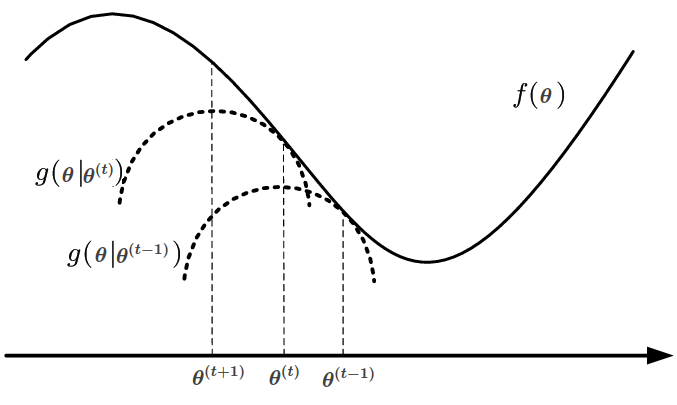
\[f(\boldsymbol{\theta^{(t + 1)}}) \overset{(1)}{\geq} g(\boldsymbol{\theta^{(t + 1)}} \mid \boldsymbol{\theta^{(t)}}) \overset{\boldsymbol{\theta^{(t + 1)} \text{ maximizer of } g(\boldsymbol{\theta} \mid \boldsymbol{\theta^{(t)}}) }}{\geq} g(\boldsymbol{\theta^{(t)}} \mid \boldsymbol{\theta^{(t)}}) \overset{(2)}{=} f(\boldsymbol{\theta^{(t)}}) \tag{3}\]The MM iterative process can be visualised in the figure below (adapted from [3] for consistent notation). The surrogate at step \(t - 1\) is the quadratic \(g(\boldsymbol{\theta} \mid \boldsymbol{\theta^{(t - 1)}})\), which is tangent to \(f\) at \(\boldsymbol{\theta^{t - 1}}\). The next estimate \(\boldsymbol{\theta^{(t)}}\) is the maximizer of this quadratic. Repeatedly following this procedure leads to better and better estimates of the maximizer of \(f\).
Now, we have a general recipe for solving hard optimization problems, but we still haven’t discussed ways of constructing the surrogate \(g\). This article ([1]) presents several methods for minorization/majorization. Here, we will only focus on the minorizer specific to the EM algorithm.
But first, a refresher on KL divergence.
Kullback-Leibler divergence
The Kullback-Leibler divergence measures how different is a probability distribution \(P\) from another probability distribution \(Q\) defined on the same probability space \(\mathcal{X}\).
\[\text{KL}(P \mid\mid Q) = - \int_{\boldsymbol{X} \in \mathcal{X}} P(\boldsymbol{X}) \log_2 \frac{Q(\boldsymbol{X})}{P(\boldsymbol{X})} d \boldsymbol{X} \tag{4}\]Assuming that \(Q\) is an approximation of an unknown distribution \(P\), the Kullback-Leibler divergence represents the average extra information (measured in bits) needed to transmit values of \(\boldsymbol{X}\) using \(Q\) as an encoding scheme instead of \(P\):
\[\underbrace{H(P, Q)}_{\text{average information to encode X using Q instead of P}} - \underbrace{H(P)}_{\text{average information to encode X using P}} = \\ \underbrace{- \int_{\boldsymbol{X} \in \mathcal{X}} P(\boldsymbol{X}) \log_2 Q(\boldsymbol{X}) d\boldsymbol{X}}_{\text{cross-entropy between P and Q}} - \Big( \underbrace{- \int_{\boldsymbol{X} \in \mathcal{X}} P(\boldsymbol{X}) \log_2 P(\boldsymbol{X}) d\boldsymbol{X}}_{\text{entropy of P}} \Big) = \\ - \int_{\boldsymbol{X} \in \mathcal{X}} P(\boldsymbol{X}) \log_2 \frac{Q(\boldsymbol{X})}{P(\boldsymbol{X})} d \boldsymbol{X} = \\ KL(P \mid\mid Q) \tag{5}\]Intuitively, we expect the KL divergence to be non-negative, as, on average, more information is needed when using a different distribution \(Q\) to encode \(\boldsymbol{X}\) that is, in reality, distributed according to \(P\). Using the probabilistic version of Jensen’s inequality and the fact that \(\log\) is a concave function, we can see that this is indeed true:
\[KL(P \mid\mid Q) = - \int_{\boldsymbol{X} \in \mathcal{X}} P(\boldsymbol{X}) \log_2 \frac{Q(\boldsymbol{X})}{P(\boldsymbol{X})} d \boldsymbol{X} = - \mathbb{E}_{\boldsymbol{X} \sim P(\boldsymbol{X})} \Big[ \log_2 \frac{Q(\boldsymbol{X})}{P({\boldsymbol{X}})} \Big] \overset{\text{Jensen}}{\geq}\] \[- \log_2 \mathbb{E}_{\boldsymbol{X} \sim P(\boldsymbol{X})} \Big[ \frac{Q(\boldsymbol{X})}{P(\boldsymbol{X})} \Big] = - \log_2 \underbrace{\int_{\boldsymbol{X} \in \mathcal{X}} \require{cancel} \cancel{P(\boldsymbol{X})} \frac{Q(\boldsymbol{X})}{\cancel{P(\boldsymbol{X})}} d\boldsymbol{X}}_{\text{Q distribution} \implies \text{ integrates to 1}} = 0 \tag{6}\]Equality holds when the random variable under expected value in Jensen’s inequality is constant, so in this case, if \(\log_2 \frac{Q(\boldsymbol{X})}{P({\boldsymbol{X}})} = \text{constant}\), which can only happen if \(P = Q\) (almost everywhere). In the next section this inequality will be used for constructing the surrogate function in the EM algorithm.
EM algorithms
Let’s first see the EM algorithm, then understand how and why it fits into the MM framework.
EM is used for determining the parameters \(\boldsymbol{\theta}\) of a probabilistic model when optimizing \(p(\boldsymbol{X} \mid \boldsymbol{\theta})\) directly is not feasible, but optimizing the joint probability \(p(\boldsymbol{X}, \boldsymbol{Z} \mid \boldsymbol{\theta})\) of the ‘full data’, consisting of the observed data \(\boldsymbol{X}\) and the latent variable \(\boldsymbol{Z}\) is easier. A distribution over the latent variable, \(q(\boldsymbol{Z})\), is introduced. We assume that \(Z\) is a discrete random variables, otherwise the sums in the following derivations will be replaced by integrals. Then, the log likelihood of the model can be decomposed into two terms, as follows:
\[\log p(\boldsymbol{X} \mid \boldsymbol{\theta}) = \log p(\boldsymbol{X} \mid \boldsymbol{\theta}) \underbrace{\sum_{\boldsymbol{Z}} q(\boldsymbol{Z})}_{\text{q sums to 1}} = \sum_{\boldsymbol{Z}} q(\boldsymbol{Z}) \log p(\boldsymbol{X} \mid \boldsymbol{\theta}) \tag{7}\]Using the chain rule for \(p(\boldsymbol{X}, \boldsymbol{Z} \mid \boldsymbol{\theta})\), we get:
\[p(\boldsymbol{X}, \boldsymbol{Z} \mid \boldsymbol{\theta}) = p(\boldsymbol{X} \mid \boldsymbol{\theta}) p(\boldsymbol{Z} \mid \boldsymbol{X}, \boldsymbol{\theta}) \implies p(\boldsymbol{X} \mid \boldsymbol{\theta}) = \frac{p(\boldsymbol{X}, \boldsymbol{Z} \mid \boldsymbol{\theta})}{p(\boldsymbol{Z} \mid \boldsymbol{X}, \boldsymbol{\theta})} \tag{8}\]Replacing (8) back into (7), we get:
\[\log p(\boldsymbol{X} \mid \boldsymbol{\theta}) = \sum_{\boldsymbol{Z}} q(\boldsymbol{Z}) \log \frac{p(\boldsymbol{X}, \boldsymbol{Z} \mid \boldsymbol{\theta})}{p(\boldsymbol{Z} \mid \boldsymbol{X}, \boldsymbol{\theta})} = \sum_{\boldsymbol{Z}} q(\boldsymbol{Z}) \log \Bigg( \frac{p(\boldsymbol{X}, \boldsymbol{Z} \mid \boldsymbol{\theta})}{q(\boldsymbol{Z})} \frac{q(\boldsymbol{Z})}{p(\boldsymbol{Z} \mid \boldsymbol{X}, \boldsymbol{\theta})} \Bigg) =\] \[\underbrace{\sum_{\boldsymbol{Z}} q(\boldsymbol{Z}) \log \frac{p(\boldsymbol{X}, \boldsymbol{Z} \mid \boldsymbol{\theta})}{q(\boldsymbol{Z})}}_{\mathcal{L}(q, \boldsymbol{\theta})} + \Bigg( \underbrace{-\sum_{\boldsymbol{Z}} q(\boldsymbol{Z}) \log \frac{p(\boldsymbol{Z} \mid \boldsymbol{X}, \boldsymbol{\theta})}{q(\boldsymbol{Z})}}_{KL(q \mid\mid p)} \Bigg) \tag{9}\]So we managed to write the log-likelihood as follows:
\[\log p(\boldsymbol{X} \mid \boldsymbol{\theta}) = \underbrace{\mathcal{L}(q, \boldsymbol{\theta}) + KL(q \mid\mid p)}_{rhs} \tag{10}\]We can notice that the parameters of the right-hand side (\(rhs\)) of (10) are both \(q\) and \(\boldsymbol{\theta}\), so if \(q\) would be fixed, then \(rhs\) would only depend on \(\boldsymbol{\theta}\), the parameter we want to optimize. The next natural question is: is it possible to fix \(q\) such that \(rhs\) becomes a minorizer for the log-likelihood? The short answer is: yes!
First, let’s remember from (6) that the Kullback-Leibler divergence is always non-negative. Using this in (10), we can see the following inequality:
\[\mathcal{L}(q, \boldsymbol{\theta}) = \log p(\boldsymbol{X} \mid \boldsymbol{\theta}) - \underbrace{KL(q \mid\mid p)}_{\geq 0} \leq \log p(\boldsymbol{X} \mid \boldsymbol{\theta}) \tag{11}\]So the value of \(\mathcal{L}(q, \boldsymbol{\theta})\) is always smaller than the value of the log-likelihood, which is a first step towards making \(\mathcal{L}\) a minorizer for the log-likelihood. This is condition (1) that a minorizer should respect.
The next step would be to choose a \(q\) such that \(\mathcal{L}(q, \boldsymbol{\theta}) = \log p(\boldsymbol{X} \mid \boldsymbol{\theta})\) for the current estimate of \(\boldsymbol{\theta}\). Looking again at (11), we can see that this is possible if the Kullback-Leibler divergence is exactly 0. We showed above that this can happen only if \(p = q\). This is condition (2) that a minorizer should respect. With this in mind, we can now sketch our iterative algorithm for maximizing the log-likelihood:
- 1. Initialize the parameter to be optimized \(\boldsymbol{\theta}_0\) arbitrarily.
- 2. Repeat for \(i = 0, 1, ...\) (until convergence)
- 2.1. Evaluate q as the posterior distribution:
In the EM framework, this represents the E step . This guarantees that \(\mathcal{L}(q, \boldsymbol{\theta})\) is a minorizer of the log-likelihood. (Note that the old parameter estimate \(\boldsymbol{\theta_i}\) only appears in \(p\), but not explicitly in \(\mathcal{L}\), which has \(\boldsymbol{\theta}\) as a free parameter)
- 2.2. Maximize the minorizer \(\mathcal{L}(q, \boldsymbol{\theta})\) w.r.t \(\boldsymbol{\theta}\), yielding a new parameter estimate:
This is called the M step in the EM framework. Because this is the same step as in the MM algorithm, it is guaranteed that the new estimate will at least as good as the previous one.
Credits
- Bishop, Christopher M. Neural networks for pattern recognition. Oxford university press, 1995.
- Hunter, D. R., & Lange, K. (2004). A tutorial on MM algorithms. The American Statistician, 58(1), 30-37.
- Coordinated Scheduling and Spectrum Sharing via Matrix Fractional Programming - Scientific Figure on ResearchGate. Available from ResearchGate [accessed 3 Mar, 2020]