Generative methods for classification

Prerequisites

• Basic calculus (logarithm rules, computing derivatives, properties of derivatives, chain rule for derivatives)
• Linear algebra (properties of traces, matrix inverses, determinants, properties of symmetric matrices)
• Basic probability and bayesian statistics notions (prior, posterior, Bayes’ rule, joint probability, independence, probability chain rule, Gaussian distribution, categorical distribution, most of them can be found here)
• Optimization concepts (convex and concave functions, finding extrema points, method of Lagrange multipliers)
• Matrix calculus (gradients and their properties, some identities involving gradients)
• Coding in python + numpy

Table of contents

1. Probabilistic framework for generative classification
2. Normally distributed inputs
3. Maximum likelihood estimation
   1. Computing the log likelihood of the dataset
   2. Estimating the class priors
   3. Estimating the means
   4. Estimating the covariance matrices
4. Decision boundary
   1. Shape of decision boundary
   2. Decision boundary and probability plots
5. Code
6. Generative power

Probabilistic framework for generative classification

Classification is the problem of assigning a discrete label (class) to a data point. Unlike discriminant methods, where the class is assigned directly, a generative approach models the joint probability of the data:

\begin{equation} \overbrace{p(\boldsymbol{x}, y)}^{\text{joint}} = \underbrace{p(y)}_{\text{class prior}} \overbrace{p(\boldsymbol{x}\mid y)}^{\text{class conditional}} \tag{1} \end{equation}

where \(\boldsymbol{x} \in \mathbb{R}^D\) (note the usage of bold symbols for vectors) is a point to be classified and \(y \in \{1, 2, \dots K \}\) is its label, with \(K\) being the total number of classes.

Intuitively, the prior represents how often a class is expected to appear and the class conditional is the probability density function (assuming \(X\) are continous) of the data having the class indicated by y.

Using this framework, the posterior probability of each class \(k\) for a new point \(\boldsymbol{x}_{new}\) is given by Bayes’ rule:

where we used the fact that \(p(\boldsymbol{x}_{new})\) is just a scaling factor that appears in all posterior probabilities and thus can be ignored.

Now, \(\boldsymbol{x}_{new}\) will be assigned to the class which yields the highest posterior probability:

Normally distributed inputs

Up to this point, we have only established the probabilistic framework we will use, but we haven’t made any assumption about the distribution of the data within each class. We will continue by making some assumptions about the underlying distributions of the data and then estimating the parameters of these distributions.

Modelling the class priors and class conditionals

We will assume that the class conditionals are multivariate Gaussian distributions:

Because there are \(K\) classes and their probabilities sum to one, the natural choice for the class priors is a categorical distribution with parameters \(\boldsymbol{\pi} = \begin{bmatrix} \pi_1, \pi_2, \dots, \pi_K \end{bmatrix}\):

Maximum Likelihood Estimation (MLE)

Before moving on, let’s recap what we have until now: we modeled the class priors using a categorical distribution with parameters \(\boldsymbol{\pi}\) and the class conditionals using Gaussian distributions with means \(\boldsymbol{\mu}_k\) and covariance matrices \(\boldsymbol{\Sigma}_k, \forall k \in \{1, 2, \dots k \}\). However, the parameters of these distributions are not known, so we must use the dataset in order to estimate them.

Maximum Likelihood Estimation (MLE) refresher

MLE is a method for estimating the parameters \(\boldsymbol{\theta}\) of a probability distribution \(p(\boldsymbol{x} \mid \boldsymbol{\theta})\) by maximizing the likelihood function of a dataset \(\mathcal{D} = \{\boldsymbol{x}_1, \dots, \boldsymbol{x}_n\}\) consisting of \(n\) i.i.d samples:

Because it is inconvenient to maximize a function containing a product, we can make use of the fact that the logarithm function transforms products into sums and is non-decreasing, thus preserving the extrema of a function:

Usually, when \(\boldsymbol{\theta}\) is unconstrained, the maximizer of the log likelihood function is found by setting the derivative w.r.t \(\boldsymbol{\theta}\) (or gradient if working with a multidimensional parameter) to zero and proving that the maximized function is concave, which is sufficient to conclude that extrema point found is indeed a maximizer. If \(\boldsymbol{\theta}\) is constrained, then a different method such as the method of Lagrange multipliers should be used.

Modeling the joint distribution of a sample

Using the class priors and class conditionals assumed above, the joint distribution of an input and its corresponding label can be written as:

where \(I[\text{condition}]\) is the indicator function (see Iverson bracket) which evaluates to 1 only if the condition inside the brackets is true.

Computing the log likelihood of the dataset

Assuming we have a dataset consisting of N independent and identically distributed samples, \(\mathcal{D} = \{(\boldsymbol{x}_i, y_i)_{i=1}^N\}\), we can write the likelihood of the data as the product of the probabilities of all samples:

Thus, the log likelihood of the dataset will be:

Estimating \(\boldsymbol{\pi}_k\)

We first notice that \(\pi_k\) appears in the log likelihood only through the term \(\log \pi_k\), so we can ignore the other term which doesn’t depend on it:

Because the \(\pi_k\)’s are constrained such that \(\sum_{k=1}^K \pi_k = 1\) (as they are the parameters of a categorical distribution), we can use the method of Lagrange multipliers to find the maximizer of the log likelihood subject to this constraint.

We formulate the Lagrangian (which is concave in both \(\boldsymbol{\pi}\) and \(\lambda\), so the solution will be indeed a maximum):

which we can reorder a bit and unclutter by noticing that the interior sum \(\sum_{i=1}^N I[y_i = k]\) is just the number of data points which have class \(k\), which we can denote as \(N_k\):

Taking the derivative of the Lagrangian w.r.t \(\pi_j\) and setting it to zero, we obtain:

Replacing \(\pi_j\) back into the Lagrangian we obtain the dual:

We remember that \(N_k\) was the number of elements in the dataset belonging to class \(k\), so naturally the sum of all \(N_k\)’s will be \(N\), the total number of elements in the dataset. Thus, we can conclude that:

So we arrived at a simple result stating that the estimated probability for each class must be the empirical probability of that class, measured on dataset \(\mathcal{D}\).

Estimating \(\boldsymbol{\mu}_k\)

Now, we look at the log likelihood again [10] and only keep the terms containing \(\boldsymbol{\mu}_k\):

Note that the log likelihood is concave in \(\boldsymbol{\mu_k}\) (quadratic with negative coefficient), so taking the gradient w.r.t \({\boldsymbol{\mu_j}}\) and setting it to zero is sufficient to find the maximum: \(\nabla_{\boldsymbol{\mu_j}}{\log \mathcal{L}(\mathcal{D} \mid \boldsymbol{\pi}, \boldsymbol{\mu}, \boldsymbol{\Sigma})} = \sum_{i=1}^N I[y_i = j] \Big( -\frac{1}{2} 2 \boldsymbol{\Sigma}_k^{-1} (\boldsymbol{x_i} - \boldsymbol{\mu}_j) \Big) \overset{!}{=} 0 \implies\)

Again, we arrived at a very simple result: the mean of each class conditional is the empirical mean of all data points belonging to that class.

Estimating \(\boldsymbol{\Sigma}_k\)

Similarly, we find the optimal \(\boldsymbol{\Sigma_k}\) by computing the gradient of the log likelihood w.r.t \(\boldsymbol{\Sigma_k}\) and setting it to zero.

Because the function is concave in \(\boldsymbol{\Sigma_j^{-1}}\) (log determinant is concave), we can compute the gradient w.r.t \(\boldsymbol{\Sigma_j^{-1}}\) directly:

We will compute the two gradients separately. For the first one we will use the log-determinant gradient rule from the table here, coupled with the fact that \(\boldsymbol{\Sigma_k}\) is a covariance matrix, thus symmetric:

For the second one, in a similar way, if \(k \neq j\), then the gradient is 0. For \(k = j\), we can notice that the expression under the gradient is a scalar, so we can apply the trace operator on it, as \(Tr(a) = a, \forall a \in \mathbb{R}\). The trace operator has some nice properties, such as the cyclic property and allowing transposing, so using the rule for the gradient of a product of two matrices w.r.t one of the matrices (from the table here), we get:

Now, using the results (20) and (21) and plugging them into the expression of the gradient of the log likelihood w.r.t \(\boldsymbol{\Sigma_j}^{-1}\) (19), we finally get:

which is the MLE estimate of the covariance of the data points having class \(j\).

Decision boundary

Shape of decision boundary

Now, having estimated the parameters of the assumed distributions, let’s inspect the shape of the decision boundary. The decision boundary is the hypersurface separating data points from 2 different classes, let’s say class \(i\) and class \(j\), so the points on this hypersurface have equal posterior probability of being assigned to either of the two classes:

Using Bayes’ rule as in (2), we can write an equivalent condition:

Now, looking at the expression above, we can see that the decision boundary is quadratic. We’ll expand it further to see each coefficient clearly:

where

Linear Discriminant Analysis for classification

The model above might have too many parameters for some applications, so it can be simplified by assuming that the covariance matrix is the same for all classes, that is \(\boldsymbol{\Sigma_i} = \boldsymbol{\Sigma}, \forall i \in \{1, 2, \dots k\}\), in which case the decision boundary will be linear, because the \(\boldsymbol{A}\) term (26) will vanish.

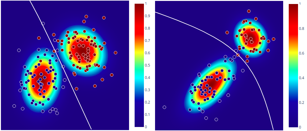
Decision boundary and probability plots

In order to visualize the decision boundary of the model, as well as the probabilities assigned by the classifier, I first generated some data using the following process:

The colour scheme in the plots encodes the probabilities assigned by the classifier to each class and the white line is the decision boundary.

For the plot on the left, I used \(\pi_1 = \pi_2 = 0.5\), means \(\boldsymbol{\mu_1} = \begin{bmatrix} 0 & 2 \end{bmatrix}^T\) (dark blue class), \(\boldsymbol{\mu_2} = \begin{bmatrix} 3 & 4 \end{bmatrix}^T\) (dark red class) and covariance matrices \(\boldsymbol{\Sigma_1} = \boldsymbol{\Sigma_2} = \begin{bmatrix} 1 & 0 \\ 0 & 1 \end{bmatrix}\). Because the model estimates different covariance matrices for different classes, we can notice that they are slightly different by looking at the shape of the contour plots (so in reality the decision boundary is ‘almost linear’). For an interactive version of the plot generated with plotly, see this.

The paramteres for the plot on the right were: \(\pi_1 = 0.6\) (dark blue class), \(\pi_2 = 0.4\) (dark red class), \(\boldsymbol{\mu_1} = \begin{bmatrix} 0 & 2 \end{bmatrix}^T\), \(\boldsymbol{\mu_1} = \begin{bmatrix} 0 & 1 \end{bmatrix}^T\), \(\boldsymbol{\mu_2} = \begin{bmatrix} 4 & 5 \end{bmatrix}^T\), \(\boldsymbol{\Sigma_1} = \begin{bmatrix} 2.5 & 2 \\ 2 & 3 \end{bmatrix}\) and \(\boldsymbol{\Sigma_2} = \begin{bmatrix} 1 & 0 \\ 0 & 1 \end{bmatrix}\). An interactive version is here.

Code

import numpy as np
from plotly import subplots
import plotly.graph_objs as go
import plotly.offline as py
from scipy.stats import multivariate_normal as gaussian


class GenerativeGaussianClassifier(object):
  def __init__(self, K):
    """Initialize a generative classifier for Gaussian inputs. 

    Parameters
    ----------
    K: int, the number of classes
    """
    self.K = K

  def fit(self, Xs, ys):
    """Estimate the parameters of the model.
    
    Fit a categorical with K classes (self.pis) representing the
    class priors and K Gaussians (with means self.mus and covariances
    self.gammas) as class conditionals.

    Parameters
    ----------
    Xs: np.ndarray of inputs having shape (num_samples, sample_size)
    ys: np.ndarray of labels having shape (num_samples, )
    """
    cls_counts = np.bincount(ys)
    get_mean = lambda k: Xs[ys == k].mean(0)
    get_cov = lambda k: np.dot((Xs[ys == k] - self.mus[k]).T, \
    	                        Xs[ys == k] - self.mus[k]) / cls_counts[k]
    get_cls_cond = lambda k: gaussian(mean=self.mus[k], cov=self.gammas[k])

    self.pis = cls_counts / len(ys)
    self.mus = np.stack([get_mean(k) for k in range(self.K)])
    self.gammas = np.stack([get_cov(k) for k in range(self.K)])
    self.cls_cond = [get_cls_cond(k) for k in range(self.K)]
	
  def predict_scores(self, Xs):
    """Use the fitted classifier to predict scores for new data.

    Parameters
    ----------
    Xs: np.ndarray of inputs having shape (num_samples, sample_size)

    Returns
    -------
    scores: np.ndarray of unnormalized scores (not probabilities)
    """
    scores = np.zeros((len(Xs), self.K), float)
    comp_score = lambda k, X: self.pis[k] * self.cls_cond[k].pdf(X)
    for i in range(len(Xs)):
      scores[i] = np.stack([comp_score(k, Xs[i]) for k in range(self.K)])
    return scores

  def predict(self, Xs):
    """Predict labels for new data.

    For each input in Xs, return a number between 0 and K - 1
    representing the class it was assigned to.

    Parameters
    ----------
    Xs: np.ndarray of inputs having shape (num_samples, sample_size)

    Returns
    -------
    labels: np.ndarray of predictions having shape (num_samples, )
    """
    labels = np.argmax(self.predict_scores(Xs), axis=1)
    return labels

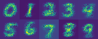
Generative power

After fitting a model, it can also be used to generate new data points. This is, however, problematic in some situations, as the estimated covariance matrix might be singular when the data actually lives in a lower dimensional subspace. It wouldn’t be very exciting to illustrate the generative power of these models on the example above, as it will simply generate points according to the 2 distributions encoded in the colours of the plot. Instead, we will look at a model fitted on MNIST digits, but a simplified version (named Naive Bayes) in which all features of a data point are assumed independent. Here, a univariate Gaussian is fitted for every pixel.

Code

import numpy as np
import matplotlib.pyplot as plt
from mnist import MNIST

mndata = MNIST('./mnist/')
Xs, ys = mndata.load_training()
Xs = np.array(Xs).astype(float) / 255.
ys = np.array(ys)

# Increase image contrast.
Xs = (Xs - Xs.min(axis=0)) / (Xs.max(axis=0) - Xs.min(axis=0) + 1e-5)

# Estimate mean and variance for each pixel.
mus = np.stack([Xs[ys == k].mean(axis=0) for k in range(10)])
var = np.stack([Xs[ys == k].var(axis=0) for k in range(10)])

# Generate a new sample from a random class.
y = np.random.choice(10)
random_sample = np.stack([np.random.normal(mus[y][i], var[y][i]) \
                          for i in range(Xs.shape[1])])

plt.imshow(random_sample.reshape(28, 28))
plt.title('Generated image from class ' + str(y))
plt.show()

Generated samples

The generated samples look pretty reasonable for such a simple model and a few lines of code!

Credits

1. Bishop, Christopher M. Neural networks for pattern recognition. Oxford university press, 1995.
2. Decision boundaries visualised via python plotly